用TensorFlow实现戴明回归算法的示例


本文摘自php中文网,作者不言,侵删。

这篇文章主要介绍了关于用TensorFlow实现戴明回归算法的示例,有着一定的参考价值,现在分享给大家,有需要的朋友可以参考一下

如果最小二乘线性回归算法最小化到回归直线的竖直距离(即,平行于y轴方向),则戴明回归最小化到回归直线的总距离(即,垂直于回归直线)。其最小化x值和y值两个方向的误差,具体的对比图如下图。


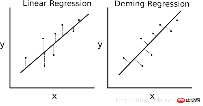
线性回归算法和戴明回归算法的区别。左边的线性回归最小化到回归直线的竖直距离;右边的戴明回归最小化到回归直线的总距离。

线性回归算法的损失函数最小化竖直距离;而这里需要最小化总距离。给定直线的斜率和截距,则求解一个点到直线的垂直距离有已知的几何公式。代入几何公式并使TensorFlow最小化距离。

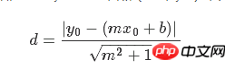
损失函数是由分子和分母组成的几何公式。给定直线y=mx+b,点(x0,y0),则求两者间的距离的公式为:

1

2

3

4

5

6

7

8

9

10

11

12

13

14

15

16

17

18

19

20

21

22

23

24

25

26

27

28

29

30

31

32

33

34

35

36

37

38

39

40

41

42

43

44

45

46

47

48

49

50

51

52

53

54

55

56

57

58

59

60

61

62

63

64

65

66

67

68

69

70

71

72

73

74

75

76

77

78

79

80

81

82

83

84

85

86

87

88

89

90

91
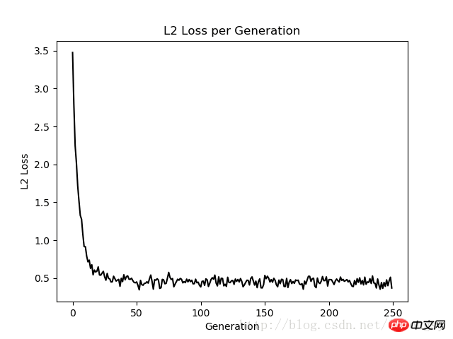
# 戴明回归

#----------------------------------

#

# This function shows how to use TensorFlow to

# solve linear Deming regression.

# y = Ax + b

#

# We will use the iris data, specifically:

# y = Sepal Length

# x = Petal Width


import matplotlib.pyplot as plt

import numpy as np

import tensorflow as tf

from sklearn import datasets

from tensorflow.python.framework import ops

ops.reset_default_graph()


# Create graph

sess = tf.Session()


# Load the data

# iris.data = [(Sepal Length, Sepal Width, Petal Length, Petal Width)]

iris = datasets.load_iris()

x_vals = np.array([x[3] for x in iris.data])

y_vals = np.array([y[0] for y in iris.data])


# Declare batch size

batch_size = 50


# Initialize placeholders

x_data = tf.placeholder(shape=[None, 1], dtype=tf.float32)

y_target = tf.placeholder(shape=[None, 1], dtype=tf.float32)


# Create variables for linear regression

A = tf.Variable(tf.random_normal(shape=[1,1]))

b = tf.Variable(tf.random_normal(shape=[1,1]))


# Declare model operations

model_output = tf.add(tf.matmul(x_data, A), b)


# Declare Demming loss function

demming_numerator = tf.abs(tf.subtract(y_target, tf.add(tf.matmul(x_data, A), b)))

demming_denominator = tf.sqrt(tf.add(tf.square(A),1))

loss = tf.reduce_mean(tf.truep(demming_numerator, demming_denominator))


# Declare optimizer

my_opt = tf.train.GradientDescentOptimizer(0.1)

train_step = my_opt.minimize(loss)


# Initialize variables

init = tf.global_variables_initializer()

sess.run(init)


# Training loop

loss_vec = []

for i in range(250):

  rand_index = np.random.choice(len(x_vals), size=batch_size)

  rand_x = np.transpose([x_vals[rand_index]])

  rand_y = np.transpose([y_vals[rand_index]])

  sess.run(train_step, feed_dict={x_data: rand_x, y_target: rand_y})

  temp_loss = sess.run(loss, feed_dict={x_data: rand_x, y_target: rand_y})

  loss_vec.append(temp_loss)

  if (i+1)%50==0:

    print('Step #' + str(i+1) + ' A = ' + str(sess.run(A)) + ' b = ' + str(sess.run(b)))

    print('Loss = ' + str(temp_loss))


# Get the optimal coefficients

[slope] = sess.run(A)

[y_intercept] = sess.run(b)


# Get best fit line

best_fit = []

for i in x_vals:

 best_fit.append(slope*i+y_intercept)


# Plot the result

plt.plot(x_vals, y_vals, 'o', label='Data Points')

plt.plot(x_vals, best_fit, 'r-', label='Best fit line', linewidth=3)

plt.legend(loc='upper left')

plt.title('Sepal Length vs Pedal Width')

plt.xlabel('Pedal Width')

plt.ylabel('Sepal Length')

plt.show()


# Plot loss over time

plt.plot(loss_vec, 'k-')

plt.title('L2 Loss per Generation')

plt.xlabel('Generation')

plt.ylabel('L2 Loss')

plt.show()

结果:


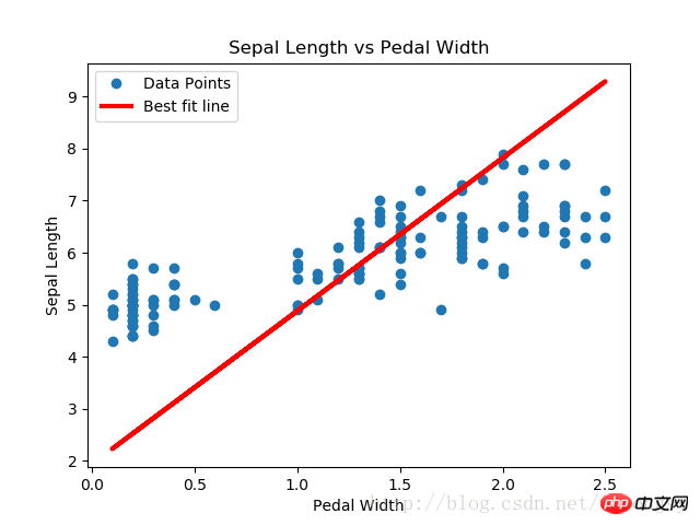
本文的戴明回归算法与线性回归算法得到的结果基本一致。两者之间的关键不同点在于预测值与数据点间的损失函数度量:线性回归算法的损失函数是竖直距离损失;而戴明回归算法是垂直距离损失(到x轴和y轴的总距离损失)。

注意,这里戴明回归算法的实现类型是总体回归(总的最小二乘法误差)。总体回归算法是假设x值和y值的误差是相似的。我们也可以根据不同的理念使用不同的误差来扩展x轴和y轴的距离计算。

相关推荐:

用TensorFlow实现多类支持向量机的示例代码

TensorFlow实现非线性支持向量机的实现方法

以上就是用TensorFlow实现戴明回归算法的示例的详细内容,更多文章请关注木庄网络博客!!

相关阅读 >>

Python目录如何修改(实例解析)

Python怎么安装turtle

Python如何调用c语言函数的使用详解

Python 创建空的list,以及append用法讲解

Python如何注释多行

Python和spyder的区别

Python的编写规范和命名规范的总结

Python的collection模块

Python的环境配置解析

Python生成任意范围任意精度的随机数的方法

更多相关阅读请进入《Python》频道 >>


打赏

取消

感谢您的支持,我会继续努力的!

扫码支持
扫码打赏,您说多少就多少

打开支付宝扫一扫,即可进行扫码打赏哦

分享从这里开始,精彩与您同在

评论

管理员已关闭评论功能...